Usage examples for Python
Get and show an image
Following Python script is the simplest usage example of
the API to get and show an image. Each method’s default value
is used if the user doesn’t input as argument. If you get ssl error,
please set ssl_verify to False.
# Load module
from jaxa.earth import je

# Get an image
data = je.ImageCollection(ssl_verify=True)\
         .filter_date()\
         .filter_resolution()\
         .filter_bounds()\
         .select()\
         .get_images()

# Process and show an image
img = je.ImageProcess(data)\
        .show_images()
A following image will be shown.
If you would like to get raw numpy array and show it, please execute following script.
import matplotlib.pyplot as plt
plt.imshow(img.raster.img[0])
plt.show()
A following image will be shown.
Search collection’s ID and Band
If you would like to know all collection’s ID and Band, please check the following page.
https://data.earth.jaxa.jp/en/datasets/
By putting a list of keywords into a method filter_name of the class ImageCollectionList,
you can easily search and identify the formal ID and band of the collection.
An example of retrieving and displaying the full list of collections and bands is as follows.:
# Load module
from jaxa.earth import je

# Get all collections and bands
collections,bands = je.ImageCollectionList(ssl_verify=True)\
                    .filter_name()

# Select a collection,band index as you like
collection_index = 0
band_index       = 0

# Get collection id and band
collection = collections[collection_index]
band       = bands[collection_index][band_index]

# Print
print(f" - collection : {collection}, band : {band}")
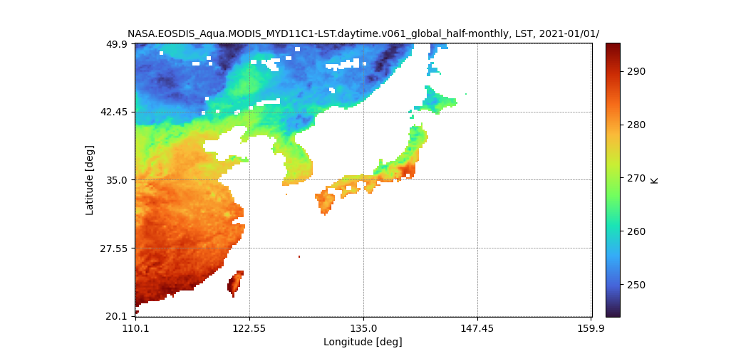
Get and show an image by region of interest
Next, set each parameter such as kw (keyword to detect collection from collection’s id), dlim (date limit), ppu (pixels per unit(one degree)).
Set region of interest by bbox
If you set bbox (bounding box), requested area will be shown.
# Load module
from jaxa.earth import je

# Set query parameters
dlim = ["2021-01-01T00:00:00","2021-01-01T00:00:00"]
ppu  = 5
bbox = [110, 20, 160, 50]

# Set information of collections,bands
collection = "NASA.EOSDIS_Terra.MODIS_MOD11C1-LST.daytime.v061_global_half-monthly"
band       = "LST"

# Get an image
data = je.ImageCollection(collection=collection,ssl_verify=True)\
        .filter_date(dlim=dlim)\
        .filter_resolution(ppu=ppu)\
        .filter_bounds(bbox=bbox)\
        .select(band=band)\
        .get_images()

# Process and show an image
img = je.ImageProcess(data)\
        .show_images()
A following image will be shown.
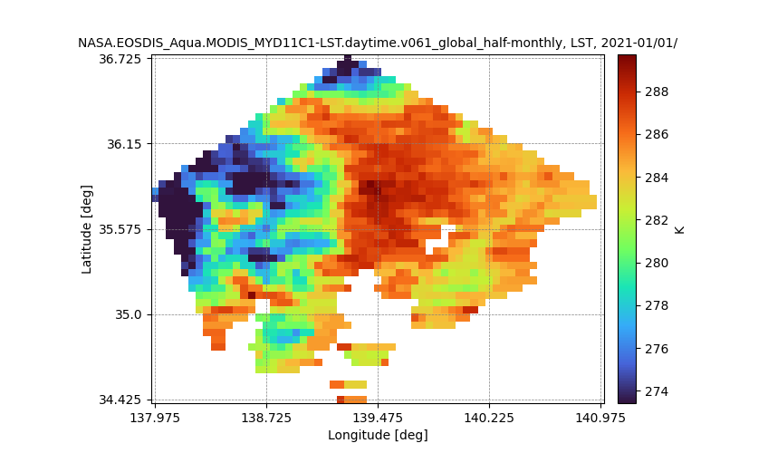
Set region of interest by geojson
If you read and set geojson data from your computer, requested area will be shown. Users can create geojson data in web service (geojson.io) or convert from another vector format such as shape file in QGIS.
# Load module
from jaxa.earth import je

# Set query parameters
dlim = ["2021-01-01T00:00:00","2021-01-01T00:00:00"]
ppu  = 20

# Set information of collection,band
collection = "NASA.EOSDIS_Aqua.MODIS_MYD11C1-LST.daytime.v061_global_half-monthly-normal"
band       = "LST_2012_2021"

# Get feature collection data
geoj_path = "test.geojson"
geoj = je.FeatureCollection().read(geoj_path).select()

# Get an image
data = je.ImageCollection(collection=collection,ssl_verify=True)\
        .filter_date(dlim=dlim)\
        .filter_resolution(ppu=ppu)\
        .filter_bounds(geoj=geoj[0])\
        .select(band=band)\
        .get_images()

# Process and show an image
img = je.ImageProcess(data)\
        .show_images()
A following image will be shown.
Get and show a masked image
Next, let’s use ImageProcess class object’s method mask_images to
mask data. Two kinds of data (mask and data to be masked) needs to be acquired.
Extract range data pixels
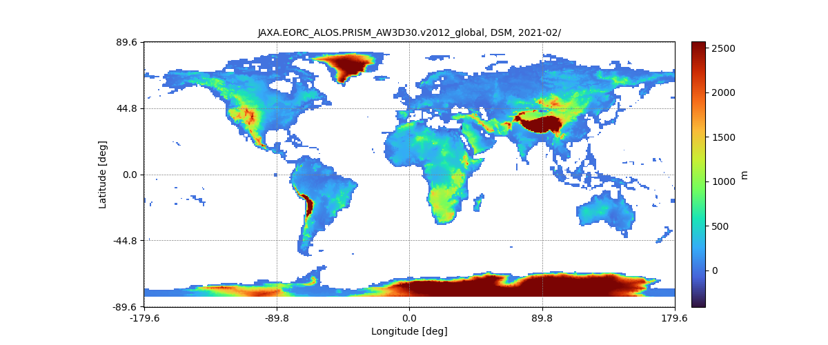
In this example, GSMaP (Monthly Rain rate) is used as data and; AW3D DSM (Elevation) is used as masking. GSMaP data is extracted by AW3D’s range from 0.01 to 1000.
# Load module
from jaxa.earth import je

# Set query parameters
dlim = ["2021-02-01T00:00:00","2021-02-01T00:00:00"]
ppu  = 10
bbox = [110, 20, 160, 50]
mq   = "range"
val  = [0.1,1000]

# Set information of collection,band for data
collection_d = "JAXA.EORC_GSMaP_standard.Gauge.00Z-23Z.v6_half-monthly-normal"
band_d       = "PRECIP_2012_2021"

# Get an image for data
data_d = je.ImageCollection(collection=collection_d,ssl_verify=True)\
        .filter_date(dlim=dlim)\
        .filter_resolution(ppu=ppu)\
        .filter_bounds(bbox=bbox)\
        .select(band=band_d)\
        .get_images()

# Get information of collections,bands for mask
collection_m = "JAXA.EORC_ALOS.PRISM_AW3D30.v3.2_global"
band_m       = "DSM"

# Get an image for mask
data_m = je.ImageCollection(collection=collection_m,ssl_verify=True)\
        .filter_date(dlim=dlim)\
        .filter_resolution(ppu=ppu)\
        .filter_bounds(bbox=bbox)\
        .select(band=band_m)\
        .get_images()

# Process and show an image
img = je.ImageProcess(data_d)\
        .mask_images(data_m,method_query=mq, values=val)\
        .show_images()
A following image will be shown.
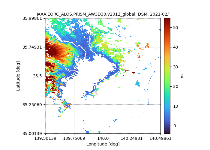
Extract values equal data pixels
In this example, AW3D DSM (Elevation) is used as data and; LCCS (Land cover) is used as masking. AW3D data is extracted by LCCS values of 190 (Urban areas).
# Load module
from jaxa.earth import je

# Set query parameters
dlim = ["2019-01-01T00:00:00","2021-02-01T00:00:00"]
ppu  = 360
bbox = [139.5, 35, 140.5, 36]
mq   = "values_equal"
val  = [190]

# Set information of collection,band for data
collection_d = "JAXA.EORC_ALOS.PRISM_AW3D30.v3.2_global"
band_d       = "DSM"

# Get an image for data
data_d = je.ImageCollection(collection=collection_d,ssl_verify=True)\
        .filter_date(dlim=dlim)\
        .filter_resolution(ppu=ppu)\
        .filter_bounds(bbox=bbox)\
        .select(band=band_d)\
        .get_images()

# Set information of collection,band for mask
collection_m = "Copernicus.C3S_PROBA-V_LCCS_global_yearly"
band_m       = "LCCS"

# Get an image for mask
data_m = je.ImageCollection(collection=collection_m,ssl_verify=True)\
        .filter_date(dlim=dlim)\
        .filter_resolution(ppu=ppu)\
        .filter_bounds(bbox=bbox)\
        .select(band=band_m)\
        .get_images()

# Process and show an image
img = je.ImageProcess(data_d)\
        .mask_images(data_m,method_query=mq, values=val)\
        .show_images()
A following image will be shown.
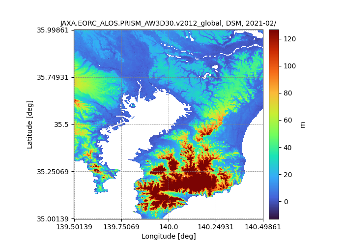
Extract bits equal data pixels
In this example, AW3D DSM (Elevation) and MSK(Mask) are used as data and mask. AW3D data band has two bands such as DSM(Elevation) and MSK (Mask). DSM is extracted by MSK bits of all zero (effective pixels).
# Load module
from jaxa.earth import je

# Set query parameters
dlim = ["2019-01-01T00:00:00","2021-02-01T00:00:00"]
ppu  = 360
bbox = [139.5, 35, 140.5, 36]
mq   = "bits_equal"
val  = [0,0,0,0,0,0,0,0]

# Set information of collection,band for data, mask
collection = "JAXA.EORC_ALOS.PRISM_AW3D30.v3.2_global"
band_d = "DSM"
band_m = "MSK"

# Get an image for data
data_d = je.ImageCollection(collection=collection,ssl_verify=True)\
        .filter_date(dlim=dlim)\
        .filter_resolution(ppu=ppu)\
        .filter_bounds(bbox=bbox)\
        .select(band=band_d)\
        .get_images()

# Get an image for mask
data_m = je.ImageCollection(collection=collection,ssl_verify=True)\
        .filter_date(dlim=dlim)\
        .filter_resolution(ppu=ppu)\
        .filter_bounds(bbox=bbox)\
        .select(band=band_m)\
        .get_images()

# Process and show an image
img = je.ImageProcess(data_d)\
        .mask_images(data_m,method_query=mq, values=val)\
        .show_images()
A following image will be shown.
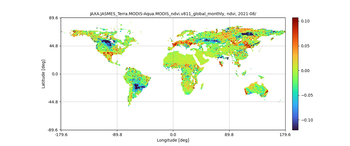
Get and show a differential image
Next, let’s use ImageProcess class object’s method diff_images to
get differential data. Two kind of data (data and reference) needs to be acquired.
In this example, NDVI (Aqua, monthly) is used as data and; NDVI (Aqua, monthly-normal) is
used as reference.
# Load module
from jaxa.earth import je

# Set query parameters
dlim = ["2021-08-01T00:00:00","2021-08-01T00:00:00"]
bbox = [-180, -90, 180, 90]

# Set information of collection,band for data
collection_d = "JAXA.JASMES_Terra.MODIS-Aqua.MODIS_ndvi.v811_global_monthly"
band_d       = "ndvi"

# Get an image for data
data_d = je.ImageCollection(collection=collection_d,ssl_verify=True)\
        .filter_date(dlim=dlim)\
        .filter_resolution()\
        .filter_bounds(bbox=bbox)\
        .select(band=band_d)\
        .get_images()

# Set information of collection,band for reference
collection_r = "JAXA.JASMES_Terra.MODIS-Aqua.MODIS_ndvi.v811_global_monthly-normal"
band_r       = "ndvi_2012_2021"

# Get an image for reference
data_r = je.ImageCollection(collection=collection_r,ssl_verify=True)\
        .filter_date(dlim=dlim)\
        .filter_resolution()\
        .filter_bounds(bbox=bbox)\
        .select(band=band_r)\
        .get_images()

# Process and show an image
img = je.ImageProcess(data_d)\
        .diff_images(data_r)\
        .show_images()
A following image will be shown.
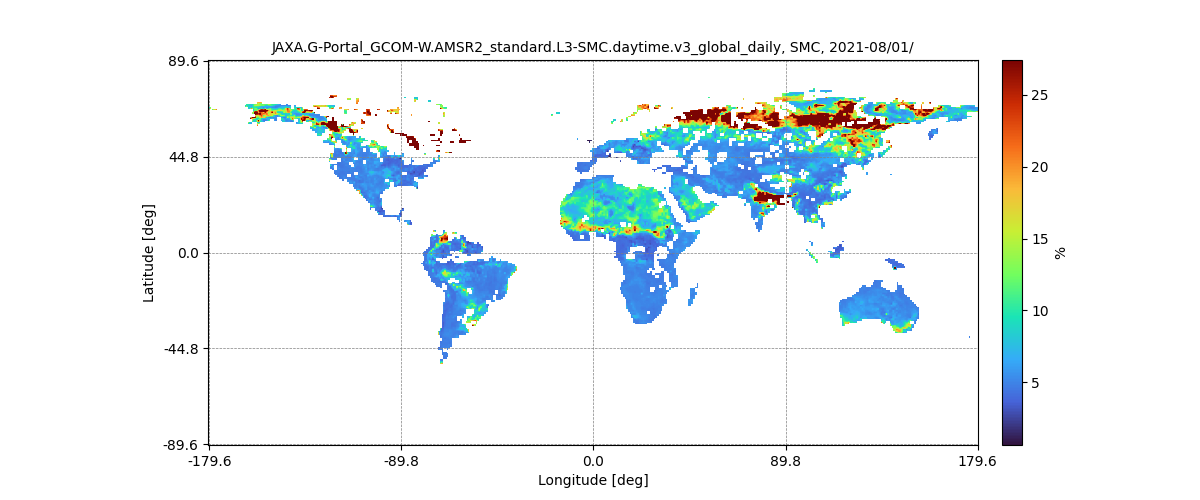
Get and show a composite image
Next, let’s use ImageProcess class object’s method calc_temporal_stats to
get a composite image. In this example, SMC (Soil Moisture Content, daily) is used
to be composite.
# Load module
from jaxa.earth import je

# Set query parameters
dlim = ["2021-08-01T00:00:00","2021-08-10T00:00:00"]
bbox = [-180, -90, 180, 90]

# Set information of collection,band for data
collection = "JAXA.G-Portal_GCOM-W.AMSR2_standard.L3-SMC.daytime.v3_global_daily"
band       = "SMC"

# Get an image for data
data = je.ImageCollection(collection=collection,ssl_verify=True)\
        .filter_date(dlim=dlim)\
        .filter_resolution()\
        .filter_bounds(bbox=bbox)\
        .select(band=band)\
        .get_images()

# Process and show an image
img = je.ImageProcess(data)\
        .calc_temporal_stats("mean")\
        .show_images()
A following image will be shown.
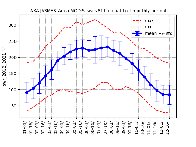
Calculate and show timeseries data
Finally, let’s use ImageProcess class object’s method calc_spatial_stats
and show_spatial_stats to calculate and show spatial statistics.
In this example, swr (Short Wave Radiation, half-monthly-normal) is used.
# Load module
from jaxa.earth import je

# Set query parameters
dlim = ["2021-01-01T00:00:00","2021-12-31T00:00:00"]
bbox = [120,20,150,50]
ppu  = 10

# Get information of collections,bands for data
collection = "JAXA.JASMES_Aqua.MODIS_swr.v811_global_half-monthly-normal"
band       = "swr_2012_2021"

# Get an image for data
data = je.ImageCollection(collection=collection,ssl_verify=True)\
        .filter_date(dlim=dlim)\
        .filter_resolution(ppu=ppu)\
        .filter_bounds(bbox=bbox)\
        .select(band=band)\
        .get_images()

# Process and show an image
img = je.ImageProcess(data)\
        .calc_spatial_stats()\
        .show_spatial_stats()

# Print timeseries numpy array
print(img.timeseries["mean"])
print(img.timeseries["std"])
print(img.timeseries["min"])
print(img.timeseries["max"])
print(img.timeseries["median"])
A following time series graph will be shown.