Pythonでの使用例

画像を取得して表示する

次のPythonスクリプトは、画像を取得して表示するというAPIの中で最も簡易的な使用例です。ユーザーが引数を入力しない場合は、各メソッドのデフォルト値が使用されます。ssl エラーが発生した場合は、ssl_verifyを False に設定してください。

# モジュールをロード
from jaxa.earth import je

# 画像を取得
data = je.ImageCollection(ssl_verify=True)\
         .filter_date()\
         .filter_resolution()\
         .filter_bounds()\
         .select()\
         .get_images()

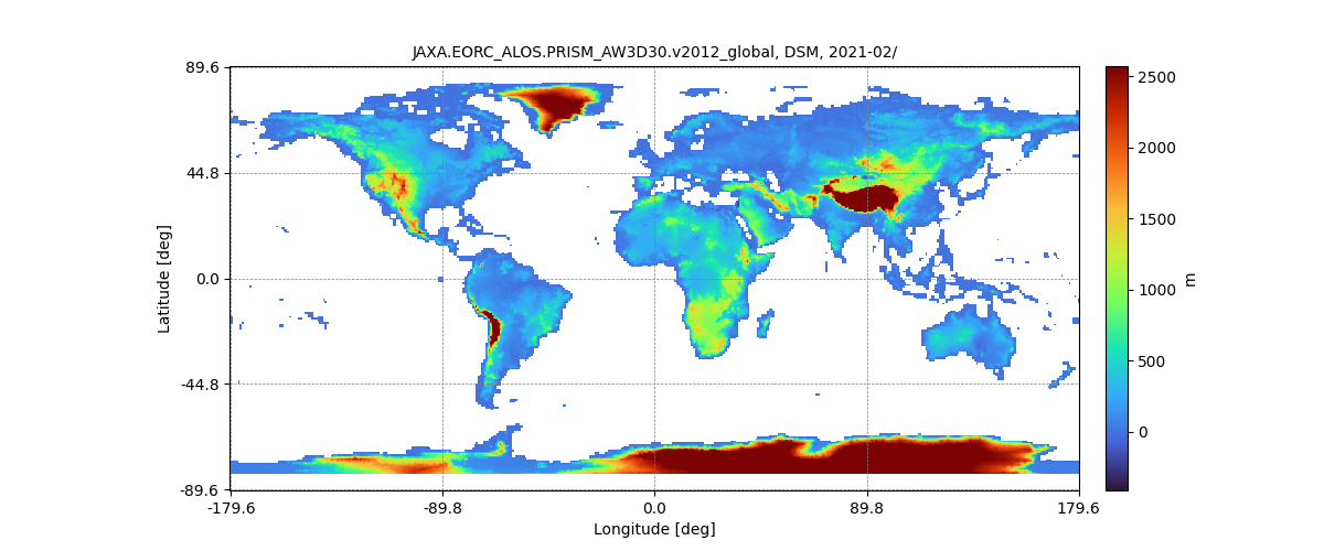
# 画像を処理して表示
img = je.ImageProcess(data)\
        .show_images()

以下の画像が表示されます。

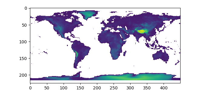
生のNumPy配列を取得して表示したい場合は、次のスクリプトを実行してください。

import matplotlib.pyplot as plt
plt.imshow(img.raster.img[0])
plt.show()

以下の画像が表示されます。

コレクションIDとバンドを検索

全てのコレクションIDとバンドを知りたい場合はこちらのページをご確認ください。

https://data.earth.jaxa.jp/en/datasets/

ImageCollectionList クラスの filter_name メソッドにキーワードのリストを入れることで、コレクションのformal IDとバンドを簡単に検索し、特定することができます。

関心領域ごとに画像を取得して表示する

次に、kw（コレクションIDからコレクションを検出するためのキーワード）、dlim（期間の範囲）、ppu（pixels per unit（1度））などの各パラメータを設定してください。

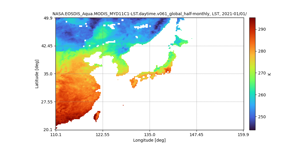
bboxによる関心領域の設定

bbox(バウンディングボックス)を設定すると、指定した領域が表示されます。

# モジュールをロード
from jaxa.earth import je

# クエリパラメータを設定
kw   = ["Aqua","LST","half-monthly"]
dlim = ["2021-01-01T00:00:00","2021-01-01T00:00:00"]
ppu  = 5
bbox = [110, 20, 160, 50]

# コレクションとバンドの情報を取得
collections,bands = je.ImageCollectionList(ssl_verify=True)\
                      .filter_name(keywords=kw)

# 画像を取得
data = je.ImageCollection(collection=collections[0],ssl_verify=True)\
         .filter_date(dlim=dlim)\
         .filter_resolution(ppu=ppu)\
         .filter_bounds(bbox=bbox)\
         .select(band=bands[0][0])\
         .get_images()

# 画像を処理して表示
img = je.ImageProcess(data)\
        .show_images()

以下の画像が表示されます。

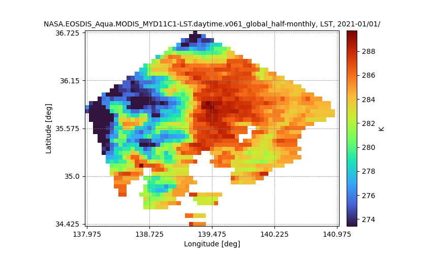
geojsonによる関心領域の設定

お使いのコンピューターからgeojsonデータを読み込んで設定すると、要求されたエリアが表示されます。ユーザーはウェブサービス（geojson.io）でgeojsonデータを作成するか、QGISでシェイプファイルなどの他のベクターフォーマットから変換することができます。

# モジュールをロード
from jaxa.earth import je

# クエリパラメータを設定
kw   = ["Aqua","LST","half-monthly"]
dlim = ["2021-01-01T00:00:00","2021-01-01T00:00:00"]
ppu  = 20

# コレクションとバンドの情報を取得
collections,bands = je.ImageCollectionList(ssl_verify=True)\
                      .filter_name(keywords=kw)

# FeatureCollectionデータを取得
geoj_path = "test.geojson"
geoj = je.FeatureCollection().read(geoj_path).select()

# 画像を取得
data = je.ImageCollection(collection=collections[0],ssl_verify=True)\
         .filter_date(dlim=dlim)\
         .filter_resolution(ppu=ppu)\
         .filter_bounds(geoj=geoj[0])\
         .select(band=bands[0][0])\
         .get_images()

# 画像を処理して表示
img = je.ImageProcess(data)\
        .show_images()

以下の画像が表示されます。

マスクされた画像を取得して表示する

次に、 ImageProcess クラスオブジェクトの mask_images メソッドを使用してデータをマスクします。マスクするデータ（マスク用データとマスクされるデータ）の2種類を取得する必要があります。

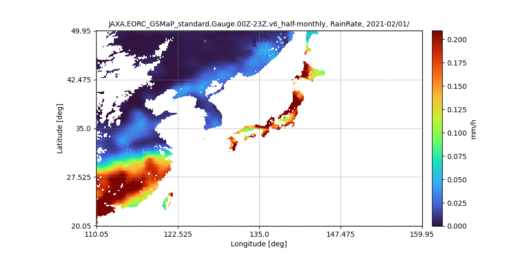
範囲データのピクセルを抽出する

次に、データとしてGSMaP (Monthly Rain rate)、マスキングにはAW3D DSM (Elevation) を使用しています。GSMaPデータは、AW3Dのrange 0.01から1000までで抽出されます。

# モジュールをロード
from jaxa.earth import je

# クエリパラメータを設定
kw_d = ["GSMaP","monthly"]
kw_m = ["AW3D"]
dlim = ["2021-02-01T00:00:00","2021-02-01T00:00:00"]
ppu  = 10
bbox = [110, 20, 160, 50]
mq   = "range"
val  = [0.1,1000]

# コレクションとバンドの情報を取得
collections_d,bands_d = je.ImageCollectionList(ssl_verify=True)\
                          .filter_name(keywords=kw_d)

# データ用の画像を取得する
data_d = je.ImageCollection(collection=collections_d[0],ssl_verify=True)\
           .filter_date(dlim=dlim)\
           .filter_resolution(ppu=ppu)\
           .filter_bounds(bbox=bbox)\
           .select(band=bands_d[0][0])\
           .get_images()

# マスク用のコレクション、バンドの情報を取得
collections_m,bands_m = je.ImageCollectionList(ssl_verify=True)\
                          .filter_name(keywords=kw_m)

# マスク用の画像の取得
data_m = je.ImageCollection(collection=collections_m[0],ssl_verify=True)\
           .filter_date(dlim=dlim)\
           .filter_resolution(ppu=ppu)\
           .filter_bounds(bbox=bbox)\
           .select(band=bands_m[0][0])\
           .get_images()

# 画像を処理して表示
img = je.ImageProcess(data_d)\
        .mask_images(data_m,method_query=mq, values=val)\
        .show_images()

以下の画像が表示されます。

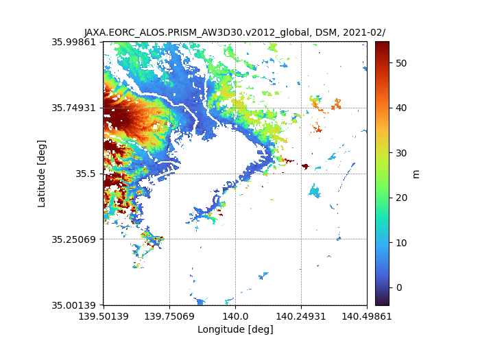
等しいデータのピクセル値を抽出する

次に、データとしてAW3D DSM (Elevation)、マスキングにはLCCS (Land cover) を使用しています。AW3Dのデータは、LCCSの190 (Urban areas)の値によって抽出されます。

# モジュールをロード
from jaxa.earth import je

# クエリパラメータを設定
kw_d = ["AW3D"]
kw_m = ["LCCS"]
dlim = ["2019-01-01T00:00:00","2021-02-01T00:00:00"]
ppu  = 360
bbox = [139.5, 35, 140.5, 36]
mq   = "values_equal"
val  = [190]

# コレクションとバンドの情報を取得
collections_d,bands_d = je.ImageCollectionList(ssl_verify=True)\
                          .filter_name(keywords=kw_d)

# データ用の画像を取得する
data_d = je.ImageCollection(collection=collections_d[0],ssl_verify=True)\
           .filter_date(dlim=dlim)\
           .filter_resolution(ppu=ppu)\
           .filter_bounds(bbox=bbox)\
           .select(band=bands_d[0][0])\
           .get_images()

# マスク用のコレクション、バンドの情報を取得
collections_m,bands_m = je.ImageCollectionList(ssl_verify=True)\
                          .filter_name(keywords=kw_m)

# マスク用の画像の取得
data_m = je.ImageCollection(collection=collections_m[0],ssl_verify=True)\
           .filter_date(dlim=dlim)\
           .filter_resolution(ppu=ppu)\
           .filter_bounds(bbox=bbox)\
           .select(band=bands_m[0][0])\
           .get_images()

# 画像を処理して表示
img = je.ImageProcess(data_d)\
        .mask_images(data_m,method_query=mq, values=val)\
        .show_images()

以下の画像が表示されます。

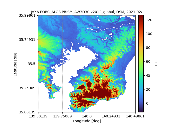
等しいビットのデータピクセルを抽出する

次に、AW3D DSM(Elevation)とMSK(Mask)がそれぞれがデータとマスクとして使用しています。AW3Dのデータバンドには、DSM(Elevation)とMSK(Mask)の2つのバンドがあります。DSMのデータは、MSKのビットが全てゼロ（有効画素数）の場合抽出されます。

# モジュールをロード
from jaxa.earth import je

# クエリパラメータを設定
kw   = ["AW3D"]
dlim = ["2019-01-01T00:00:00","2021-02-01T00:00:00"]
ppu  = 360
bbox = [139.5, 35, 140.5, 36]
mq   = "bits_equal"
val  = [0,0,0,0,0,0,0,0]

# コレクションとバンドの情報を取得
collections,bands = je.ImageCollectionList(ssl_verify=True)\
                          .filter_name(keywords=kw)

# データ用の画像を取得する
data_d = je.ImageCollection(collection=collections[0],ssl_verify=True)\
           .filter_date(dlim=dlim)\
           .filter_resolution(ppu=ppu)\
           .filter_bounds(bbox=bbox)\
           .select(band="DSM")\
           .get_images()

# マスク用の画像の取得
data_m = je.ImageCollection(collection=collections[0],ssl_verify=True)\
           .filter_date(dlim=dlim)\
           .filter_resolution(ppu=ppu)\
           .filter_bounds(bbox=bbox)\
           .select(band="MSK")\
           .get_images()

# 画像を処理して表示
img = je.ImageProcess(data_d)\
        .mask_images(data_m,method_query=mq, values=val)\
        .show_images()

以下の画像が表示されます。

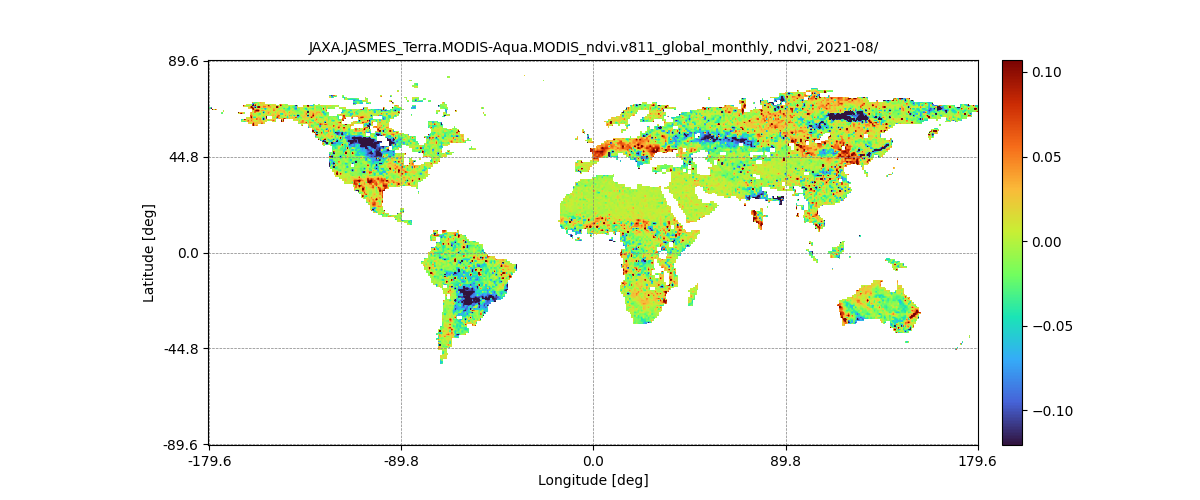
差分画像を取​​得して表示する

次に、 ImageProcess クラスの diff_images メソッドを使い、差分データを取得しています。2種類のデータ（比較対象となるデータと基準データ）を取得する必要があります。この例では対象データとしてNDVI (Aqua, monthly)、基準データとしてNDVI (Aqua, monthly-normal)を使用しています。

# モジュールをロード
from jaxa.earth import je

# クエリパラメータを設定
kw_d = ["ndvi","_monthly"]
kw_r = ["ndvi","_monthly","normal"]
dlim = ["2021-08-01T00:00:00","2021-08-01T00:00:00"]

# データ用のコレクション、バンドの情報を取得
collections_d,bands_d = je.ImageCollectionList(ssl_verify=True)\
                          .filter_name(keywords=kw_d)

# データ用の画像を取得する
data_d = je.ImageCollection(collection=collections_d[0],ssl_verify=True)\
           .filter_date(dlim=dlim)\
           .filter_resolution()\
           .filter_bounds()\
           .select(band=bands_d[0][0])\
           .get_images()

# Collectionとバンドの情報を取得
collections_r,bands_r = je.ImageCollectionList(ssl_verify=True)\
                          .filter_name(keywords=kw_r)

# 基準画像を入手する
data_r = je.ImageCollection(collection=collections_r[0],ssl_verify=True)\
           .filter_date(dlim=dlim)\
           .filter_resolution()\
           .filter_bounds()\
           .select(band=bands_r[0][0])\
           .get_images()

# 画像を処理して表示
img = je.ImageProcess(data_d)\
        .diff_images(data_r)\
        .show_images()

以下の画像が表示されます。

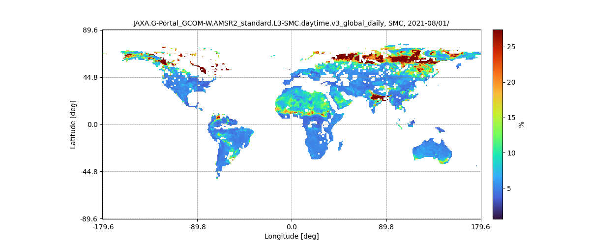
合成画像を取得して表示する

次に、 ImageProcess クラスの calc_temporal_stats メソッドを使用して、合成画像を取得しています。この例では、SMC (Soil Moisture Content, daily)が合成の対象として使用されています。

# モジュールをロード
from jaxa.earth import je

# クエリパラメータを設定
kw_d = ["SMC","_daily"]
dlim = ["2021-08-01T00:00:00","2021-08-10T00:00:00"]

# データ用のコレクション、バンドの情報を取得
collections,bands = je.ImageCollectionList(ssl_verify=True)\
                          .filter_name(keywords=kw_d)

# データ用の画像を取得する
data = je.ImageCollection(collection=collections[0],ssl_verify=True)\
           .filter_date(dlim=dlim)\
           .filter_resolution()\
           .filter_bounds()\
           .select(band=bands[0][0])\
           .get_images()

# 画像を処理して表示
img = je.ImageProcess(data)\
        .calc_temporal_stats("mean")\
        .show_images()

以下の画像が表示されます。

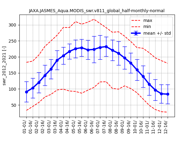
時系列データの計算と表示

最後に、 ImageProcess クラスのオブジェクトの calc_spatial_stats メソッドと show_spatial_stats メソッドを使用して、空間統計を計算し、表示します。この例では、swr (Short Wave Radiation, half-monthly-normal)を使用しています。

# モジュールをロード
from jaxa.earth import je

# クエリパラメータを設定
kw_d = ["swr","half-monthly-normal"]
dlim = ["2021-01-01T00:00:00","2021-12-31T00:00:00"]
bbox = [120,20,150,50]
ppu  = 10

# データ用のコレクション、バンドの情報を取得
collections,bands = je.ImageCollectionList(ssl_verify=True)\
                          .filter_name(keywords=kw_d)

# データ用の画像を取得する
data = je.ImageCollection(collection=collections[0],ssl_verify=True)\
           .filter_date(dlim=dlim)\
           .filter_resolution(ppu=ppu)\
           .filter_bounds(bbox=bbox)\
           .select(band=bands[0][0])\
           .get_images()

# 画像を処理して表示
img = je.ImageProcess(data)\
        .calc_spatial_stats()\
        .show_spatial_stats()

以下の時系列グラフが表示されます。