Python 使用例
画像の取得と表示
最もシンプルな使用例 — すべてデフォルト値で画像を取得・表示します:
from jaxa.earth import je

# 画像の取得
data = je.ImageCollection(ssl_verify=True) \
         .filter_date() \
         .filter_resolution() \
         .filter_bounds() \
         .select() \
         .get_images()

# 画像の処理と表示
img = je.ImageProcess(data) \
        .show_images()
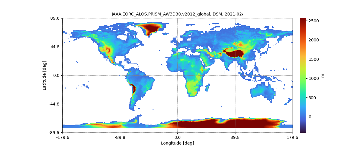
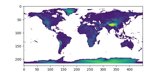
生のnumpy配列を取得して表示する場合:
コレクションIDとバンドの検索
利用可能なデータセットの一覧は https://data.earth.jaxa.jp/en/datasets/ で確認できます。
ImageCollectionList.filter_name() でキーワード検索が可能です:
from jaxa.earth import je

# 全コレクションとバンドの取得
collections, bands = je.ImageCollectionList(ssl_verify=True) \
                       .filter_name()

collection_index = 0
band_index = 0

collection = collections[collection_index]
band = bands[collection_index][band_index]
print(f" - collection : {collection}, band : {band}")
関心領域を指定した画像の取得と表示
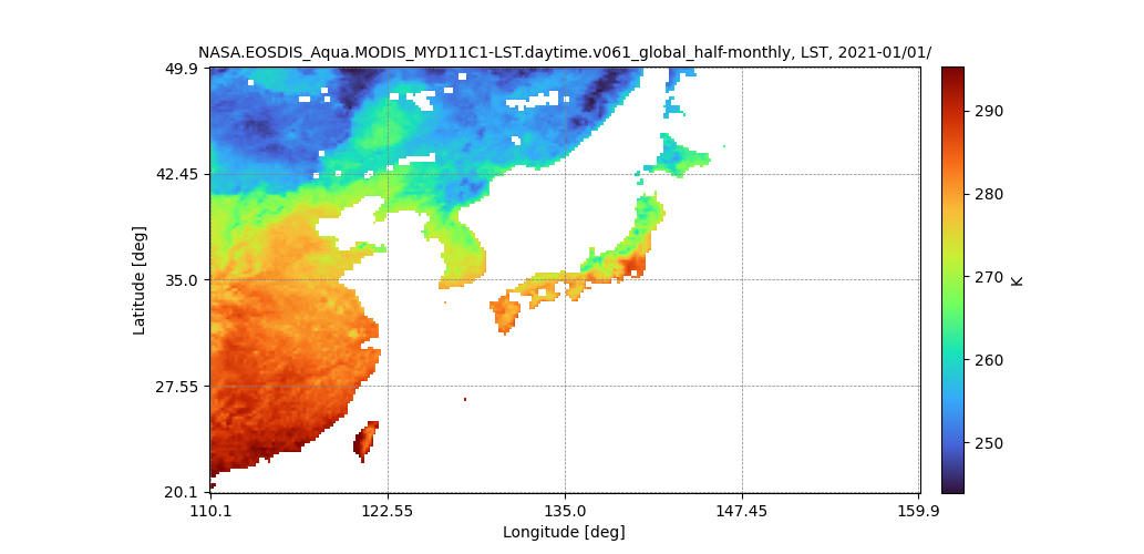
バウンディングボックスで関心領域を指定
from jaxa.earth import je

dlim       = ["2021-01-01T00:00:00","2021-01-01T00:00:00"]
ppu        = 5
bbox       = [110, 20, 160, 50]
collection = "NASA.EOSDIS_Terra.MODIS_MOD11C1-LST.daytime.v061_global_half-monthly"
band       = "LST"

data = je.ImageCollection(collection=collection, ssl_verify=True) \
         .filter_date(dlim=dlim) \
         .filter_resolution(ppu=ppu) \
         .filter_bounds(bbox=bbox) \
         .select(band=band) \
         .get_images()

img = je.ImageProcess(data) \
        .show_images()
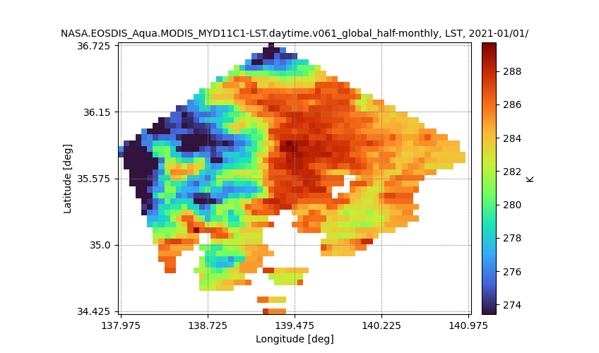
GeoJSONで関心領域を指定
GeoJSONデータは geojson.io で作成するか、QGISでシェープファイルから変換します:
from jaxa.earth import je

dlim       = ["2021-01-01T00:00:00","2021-01-01T00:00:00"]
ppu        = 20
collection = "NASA.EOSDIS_Aqua.MODIS_MYD11C1-LST.daytime.v061_global_half-monthly-normal"
band       = "LST_2012_2021"

geoj_path  = "test.geojson"
geoj       = je.FeatureCollection().read(geoj_path).select()

data = je.ImageCollection(collection=collection, ssl_verify=True) \
         .filter_date(dlim=dlim) \
         .filter_resolution(ppu=ppu) \
         .filter_bounds(geoj=geoj[0]) \
         .select(band=band) \
         .get_images()

img = je.ImageProcess(data) \
        .show_images()
マスク画像の取得と表示
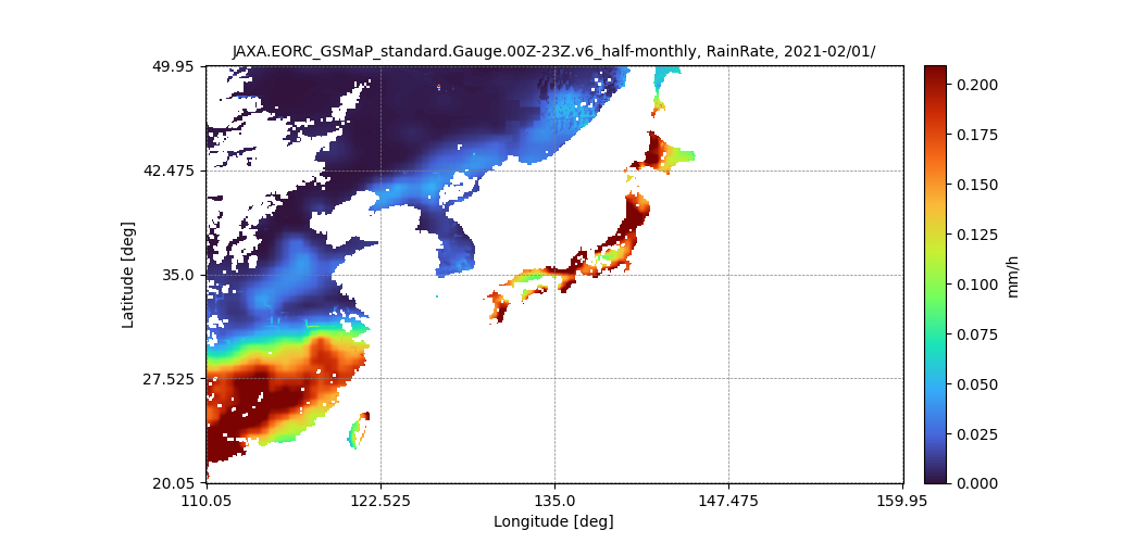
範囲データのピクセル抽出
AW3D標高範囲 [0.1, 1000] でGSMaP降水量データをマスク:
from jaxa.earth import je

dlim = ["2021-02-01T00:00:00","2021-02-01T00:00:00"]
ppu  = 10
bbox = [110, 20, 160, 50]

# データの取得
data_d = je.ImageCollection("JAXA.EORC_GSMaP_standard.Gauge.00Z-23Z.v6_half-monthly-normal", ssl_verify=True) \
           .filter_date(dlim=dlim).filter_resolution(ppu=ppu) \
           .filter_bounds(bbox=bbox).select("PRECIP_2012_2021").get_images()

# マスクの取得
data_m = je.ImageCollection("JAXA.EORC_ALOS.PRISM_AW3D30.v3.2_global", ssl_verify=True) \
           .filter_date(dlim=dlim).filter_resolution(ppu=ppu) \
           .filter_bounds(bbox=bbox).select("DSM").get_images()

# マスクの適用
img = je.ImageProcess(data_d) \
        .mask_images(data_m, method_query="range", values=[0.1, 1000]) \
        .show_images()
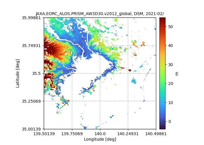
特定値のピクセル抽出
LCCS土地被覆値 190(都市域)でAW3D標高をマスク:
from jaxa.earth import je

dlim = ["2019-01-01T00:00:00","2021-02-01T00:00:00"]
ppu  = 360
bbox = [139.5, 35, 140.5, 36]

data_d = je.ImageCollection("JAXA.EORC_ALOS.PRISM_AW3D30.v3.2_global", ssl_verify=True) \
           .filter_date(dlim=dlim).filter_resolution(ppu=ppu) \
           .filter_bounds(bbox=bbox).select("DSM").get_images()

data_m = je.ImageCollection("Copernicus.C3S_PROBA-V_LCCS_global_yearly", ssl_verify=True) \
           .filter_date(dlim=dlim).filter_resolution(ppu=ppu) \
           .filter_bounds(bbox=bbox).select("LCCS").get_images()

img = je.ImageProcess(data_d) \
        .mask_images(data_m, method_query="values_equal", values=[190]) \
        .show_images()
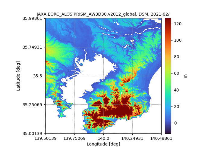
ビット値によるピクセル抽出
AW3D MSK(マスク)を使って bits_equal でDSM(標高)をマスク。全ビットゼロは有効ピクセルを意味します:
from jaxa.earth import je

dlim       = ["2019-01-01T00:00:00","2021-02-01T00:00:00"]
ppu        = 360
bbox       = [139.5, 35, 140.5, 36]
collection = "JAXA.EORC_ALOS.PRISM_AW3D30.v3.2_global"

data_d = je.ImageCollection(collection, ssl_verify=True) \
           .filter_date(dlim=dlim).filter_resolution(ppu=ppu) \
           .filter_bounds(bbox=bbox).select("DSM").get_images()

data_m = je.ImageCollection(collection, ssl_verify=True) \
           .filter_date(dlim=dlim).filter_resolution(ppu=ppu) \
           .filter_bounds(bbox=bbox).select("MSK").get_images()

img = je.ImageProcess(data_d) \
        .mask_images(data_m, method_query="bits_equal", values=[0,0,0,0,0,0,0,0]) \
        .show_images()
差分画像の取得と表示
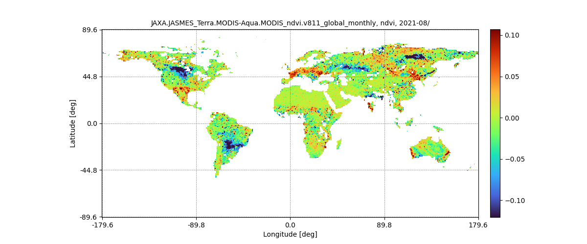
diff_images を使ってNDVI(月別)とNDVI(月別平年値)の差分画像を作成:
from jaxa.earth import je

dlim = ["2021-08-01T00:00:00","2021-08-01T00:00:00"]
bbox = [-180, -90, 180, 90]

# データ
data_d = je.ImageCollection("JAXA.JASMES_Terra.MODIS-Aqua.MODIS_ndvi.v811_global_monthly", ssl_verify=True) \
           .filter_date(dlim=dlim).filter_resolution() \
           .filter_bounds(bbox=bbox).select("ndvi").get_images()

# 参照(平年値)
data_r = je.ImageCollection("JAXA.JASMES_Terra.MODIS-Aqua.MODIS_ndvi.v811_global_monthly-normal", ssl_verify=True) \
           .filter_date(dlim=dlim).filter_resolution() \
           .filter_bounds(bbox=bbox).select("ndvi_2012_2021").get_images()

img = je.ImageProcess(data_d) \
        .diff_images(data_r) \
        .show_images()
合成画像の取得と表示
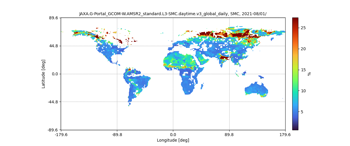
calc_temporal_stats を使って複数の日別画像を1枚に合成:
from jaxa.earth import je

dlim = ["2021-08-01T00:00:00","2021-08-10T00:00:00"]
bbox = [-180, -90, 180, 90]

data = je.ImageCollection("JAXA.G-Portal_GCOM-W.AMSR2_standard.L3-SMC.daytime.v3_global_daily", ssl_verify=True) \
         .filter_date(dlim=dlim).filter_resolution() \
         .filter_bounds(bbox=bbox).select("SMC").get_images()

img = je.ImageProcess(data) \
        .calc_temporal_stats("mean") \
        .show_images()
時系列データの計算と表示
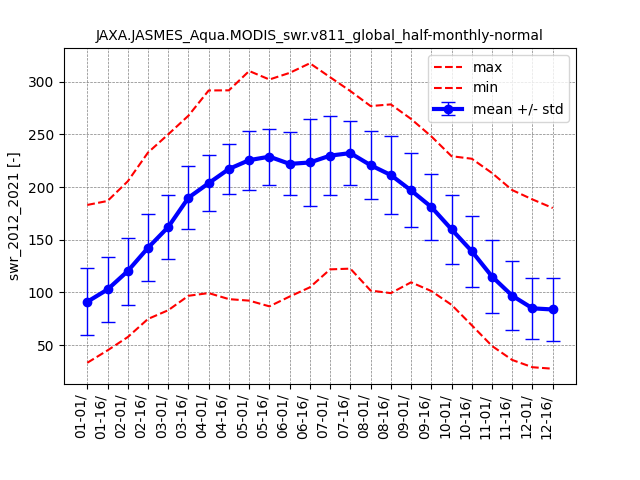
複数日付にわたる空間統計を計算し、時系列グラフとして表示:
from jaxa.earth import je

dlim       = ["2021-01-01T00:00:00","2021-12-31T00:00:00"]
bbox       = [120, 20, 150, 50]
ppu        = 10
collection = "JAXA.JASMES_Aqua.MODIS_swr.v811_global_half-monthly-normal"
band       = "swr_2012_2021"

data = je.ImageCollection(collection, ssl_verify=True) \
         .filter_date(dlim=dlim).filter_resolution(ppu=ppu) \
         .filter_bounds(bbox=bbox).select(band).get_images()

img = je.ImageProcess(data) \
        .calc_spatial_stats() \
        .show_spatial_stats()

# 時系列のnumpy配列にアクセス
print(img.timeseries["mean"])
print(img.timeseries["std"])
print(img.timeseries["min"])
print(img.timeseries["max"])
print(img.timeseries["median"])